Torsional Analysis of Rigid Diaphragm |
  
|
Torsional Analysis of Rigid Diaphragm |
|
This module analyzes the distribution of lateral forces across a rigid diaphragm, accounting for both direct shear and torsional effects. It uses a stiffness-based approach to determine how lateral loads, typically from wind or seismic forces, are transferred to each resisting element based on its position, orientation, and relative stiffness, while also accounting for accidental eccentricity between the center of mass and center of rigidity.
Limitations:
•Assumes a rigid diaphragm; flexible and semi-rigid diaphragm effects are not included.
•Supports up to 160 different force resisting elements (walls, bending elements, or generic).
•Analysis is for one diaphragm level only. Multi-level buildings require separate calculations per level.
•Results depend on accurate element locations, stiffnesses, and orientations entered by the user.
•Does not model vertical alignment (i.e. when elements are offset between levels). The center of mass must be recalculated manually for each level.
•Neglects individual resisting element local torsional stiffness (J).
Unique Features
•Automated Directional and Eccentricity Load Conditions – The module automatically evaluates all combinations of lateral load directions and accidental eccentricity positions. Lateral forces can be applied at custom angular increments (e.g., 15°, 30°), and eccentricities are resolved along an elliptical path centered at the shear application point. This produces a full set of load conditions capturing both translational and torsional effects without requiring users to manually define multiple scenarios.
•Rigorous Stiffness Analysis – This module uses a numerical, stiffness-based approach to calculate how lateral forces are distributed and how torsional effects develop. Unlike simplified methods that assume elements act only in orthogonal directions, this module supports elements oriented at any angle. Each element’s stiffness is calculated about its local principal axes, transformed into the global coordinate system, and combined with all other elements to determine the overall stiffness matrix and center of rigidity. This enables a more complete and realistic evaluation of force distribution and torsional behavior.
•Support for Multiple Element Types – Walls, bending members, and generic resisting elements can be modeled together, each with independent stiffness properties, orientations, and boundary conditions, enabling realistic simulation of complex lateral force-resisting systems.
Coordinate System
Please ensure a strict X-Y coordinate system is used for accurate analysis. When setting up the model, keep in mind that Global +X increases to the right and Global +Y increases upward on the screen.
Analysis Procedure
For more details on how the lateral force-resisting system stiffness is calculated and how forces are resolved for each resisting element, please refer to the topic: Torsional Analysis of Rigid Diaphragm Theory
Basic Usage
1.Define the Location of Shear Application: Enter the X-Y coordinates where lateral forces act on the diaphragm. These typically represent seismic or wind loads at that level. If loads from other levels contribute, combine them into a single adjusted load location before input.
2.Configure Accidental Eccentricity: To account for seismic or wind-induced torsional effects, specify the accidental eccentricity as a percentage of the building’s plan dimensions. You can also define an angular increment to control how many offset load locations (around the eccentricity ellipse) are evaluated. This enables the program to automatically generate all load conditions combining direction and eccentricity.
3.Specify Lateral Loads: Define the magnitude and direction of the diaphragm loads by choosing one of the following methods:
a.Apply a primary force alone or with an orthogonal component;
b.Resolve independent X and Y forces based on a specified load angle; or
c.Use a 100% + 30% orthogonal combination method per ASCE 7
4.Add Resisting Elements: Use the Walls, Bending Members, or Generic subtab to define each resisting element. For each:
a.Enter the X and Y coordinates of the element’s centroid, which serves as its center of rigidity.
b.Specify the orientation angle (θ) of the element’s local +y axis (strong axis), measured counterclockwise from the global +X axis.
i.Positive angles rotate counterclockwise from the global +X axis.
ii.Default orientation (θ = 0 degrees):
1.Local +y (strong axis): Parallel to global +X (points right on screen)
2.Local +x (weak axis): 90° clockwise from +y (points downward on screen)
c.Enter geometric or section properties appropriate to the element type (e.g., dimensions for walls, moments of inertia for bending members, or flexibilities for generic elements).
d.Set Elastic Modulus: If all elements are made of the same material, you may simplify input by using a relative modulus (e.g., Eb = 1). Only the relative stiffness between elements affects the analysis.
e.Define Fixity Conditions: Select the fixity condition that best represents each element’s top and bottom restraint against rotation about both the local +x and +y axes:
i.Use Fix-Pin for inverted pendulum conditions (e.g., cantilevered walls or columns with fixed bases and free tops), or for moment frames with pinned column bases.
ii.Use Fix-Fix when both ends are restrained, resulting in double curvature behavior.
5.Review Results: The module automatically generates all load conditions based on load directions and eccentricity increments. Use the result tabs to view maximum forces per element, detailed forces by load case, and stiffness or displacement matrices for verification.
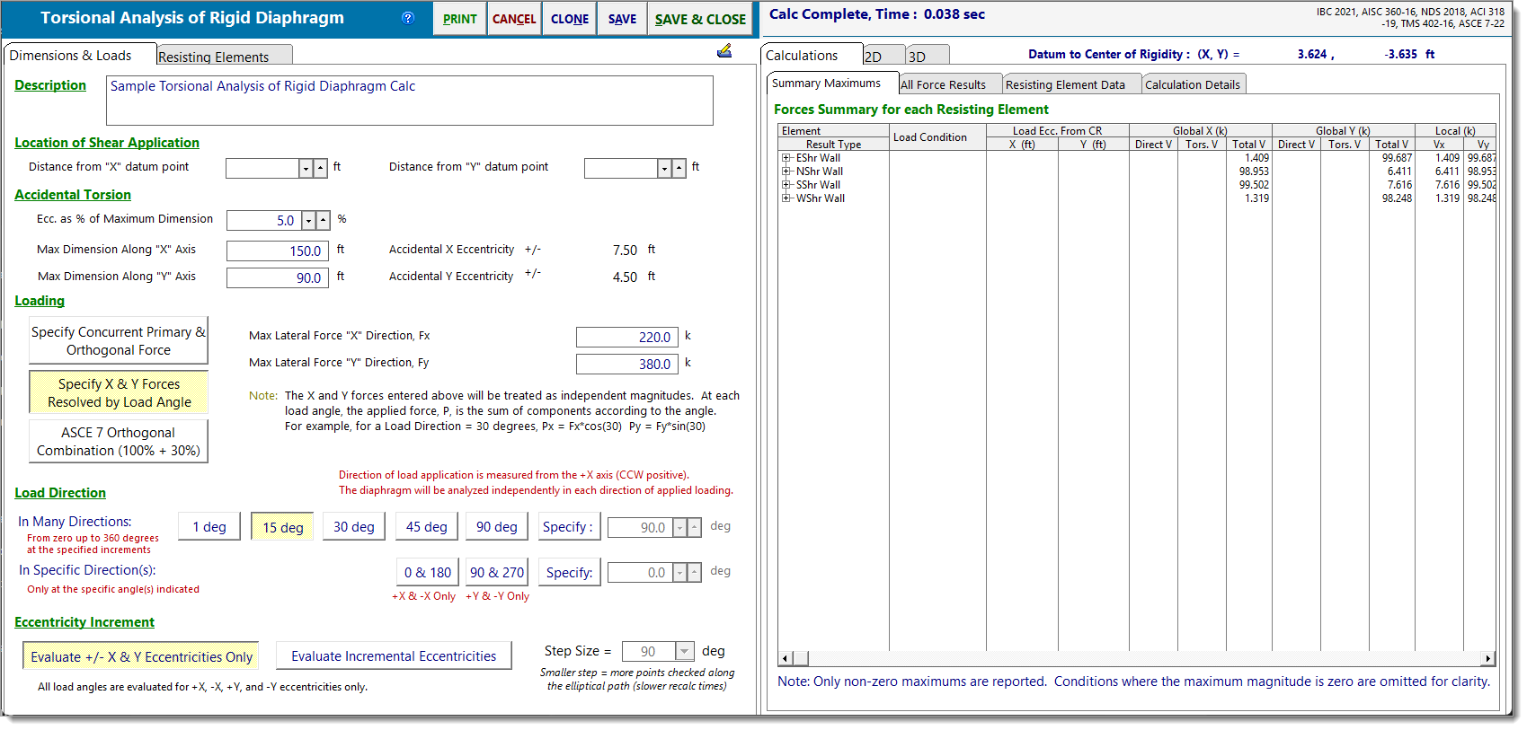
Dimensions & Loads
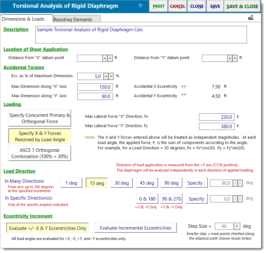
Location of Shear Application
This specifies the X-Y coordinates of the center of the load ellipse where the lateral shears act (e.g. center of mass for seismic loads, center of exposure for wind loads).
Accidental torsion accounts for uncertainty in the exact location of a structure’s center of rigidity and center of mass, which can cause additional torsion under seismic or wind loads. ASCE 7 accounts for this this by adding an accidental eccentricity; a small offset between the center of mass (for seismic loads) or center of exposure (for wind loads) and the center of rigidity, on top of any actual offset already present. This offset is typically a percentage of the overall building dimensions perpendicular to each direction.
Ecc as % of Maximum Dimension: Percent of building dimension to use for eccentricity (e.g., 5%).
Max Dimension Along "X" Axis: Plan dimension used to calculate the accidental eccentricity in the X direction.
Max Dimension Along "Y" Axis: Plan dimension used to calculate the accidental eccentricity in the Y direction.
For more information regarding how this module accounts for the accidental eccentricity in the analysis, see the sections regarding the Eccentricity Increment and How Load Direction and Eccentricity Increment Work Together.
These controls define how lateral forces are specified and combined for diaphragm loading.
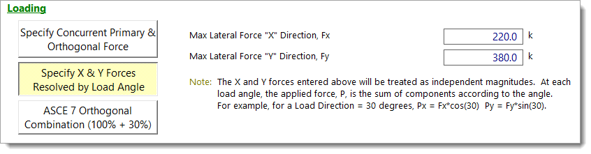
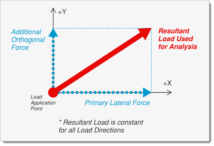
Specify Concurrent Primary & Orthogonal Force
When this option is selected, the resultant of the primary and orthogonal forces is applied to the force resisting system at the angle or angular increments defined below under Load Direction. The Resultant Load is applied to the rigid diaphragm at the various load directions and eccentricities described below.
Primary Lateral Force: This is the primary lateral force to be applied to the rigid diaphragm.
Additional Orthogonal Force: This is an optional orthogonal force that is to be applied at a 90-degree angle to the Primary Lateral Force.
Resultant Load Used for Analysis: This is the resultant force which is actually applied to the diaphragm. It is calculated as the square root of the sum of the squares of the Primary Lateral Force and the Additional Orthogonal Force.
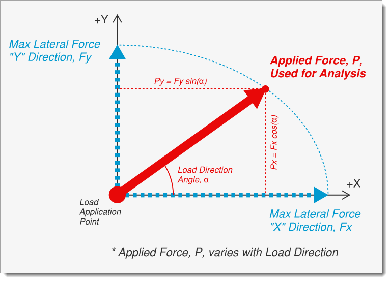
Specify X & Y Forces Resolved by Load Angle
When this option is selected, the X and Y forces will be treated as independent magnitudes. At each load angle, the applied force, P, is the vector sum of components according to the load angle. For example, for a Load Direction = 30 degrees, Px = Fx * cos(30°) and Py = Fy * sin(30°).
Max Lateral Force "X" Direction, Fx: This is the maximum lateral force in the +X & -X directions (i.e. when the load angle is exactly 0 or 180 degrees).
Max Lateral Force "Y" Direction, Fy: This is the maximum lateral force in the +Y & -Y directions (i.e. when the load angle is exactly 90 or 270 degrees).
ASCE 7 Orthogonal Combination (100% + 30%)
When this option is selected, the diaphragm is analyzed for a series of conditions where it is loaded simultaneously with 100% of lateral force in one direction and 30% of lateral force in the perpendicular direction.
Max Lateral Force "X" Direction, Fx: This is the maximum lateral force in the +X & -X directions.
Max Lateral Force "Y" Direction, Fy: This is the maximum lateral force in the +Y & -Y directions.
Conditions are permuted so that each axis experiences both +/- 100% and +/- 30% as described in the orthogonal combination procedure of ASCE 7. This results in the following 8 load conditions:
•+100% Fx + 30% Fy
•+100% Fx - 30% Fy
•-100% Fx + 30% Fy
•-100% Fx - 30% Fy
•+30% Fx + 100% Fy
•+30% Fx - 100% Fy
•-30% Fx + 100% Fy
•-30% Fx - 100% Fy
NOTE: Load Direction inputs are not applicable when the ASCE 7 Orthogonal Combination option is selected. In this case, the Load Direction controls will be disabled, and all loads will be applied parallel to the global X and Y axes of the diaphragm.
These controls determine the direction in which lateral forces are applied to the diaphragm.
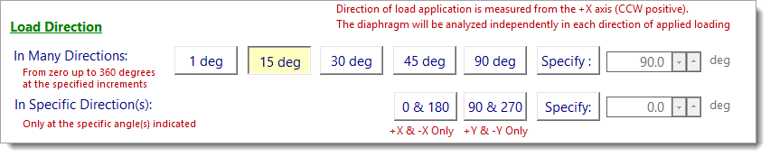
In Many Directions
Per ASCE 7, seismic forces must be applied in the directions that produce the most critical load effects. This module can satisfy that requirement by applying the specified lateral loads at multiple angles, helping to identify the true critical direction for each resisting element.
When applying loads In Many Directions, the module will apply the specified lateral forces to the diaphragm at the chosen angular increment:
•1 deg: Loads applied at 0°, 1°, 2°, etc.
•15° deg: Loads applied at 0°, 15°, 30°, etc.
•30° deg: Loads applied at 0°, 30°, 60°, etc.
•45° deg: Loads applied at 0°, 45°, 90°, etc.
•90° deg: Loads applied at 0°, 90°, 180°, etc.
•Specify: Loads at a custom increment (e.g., entering 20° applies loads at 0°, 20°, 40°, etc.).
TIP: If you would like to utilize ASCE 7's Independent Directional Procedure and only apply the loads independently in two orthogonal directions (X & Y), this can be accomplished by using the In Many Directions > 90 deg option. This applies loads to the diaphragm at 0°, 90°, 180°, and 270°, corresponding to +X, +Y, -X, and -Y directions.
In Specific Directions
Instead of testing multiple angles, you can also apply loads at specific directions only:
•0 & 180: Loads applied in +X and -X directions only.
•90 & 270: Loads applied in +Y and -Y directions only.
•Specify: Loads applied at a single user-defined angle.
NOTE: Direction of load application is measured from the +X axis (counterclockwise positive). The diaphragm will be analyzed independently in each direction of applied loading.
The magnitude of the lateral force applied to the diaphragm is determined by the previously selected Loading method. For example, if the Specify Concurrent Primary & Orthogonal Force mode is used with a 30° angular increment, the Resultant Load will be applied at 0°, 30°, 60°, and so on, continuing around the full 360° range.
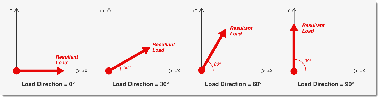
When using the Specify X & Y Forces Resolved by Load Angle Loading method with a 30° angular increment, the applied force P is computed as the vector sum of the X and Y components corresponding to each load direction angle. This process repeats at every increment from 0° through 360°.
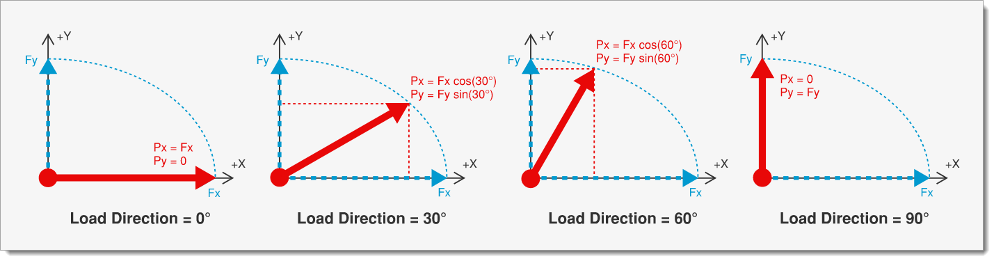
NOTE: At 0° and 180°, the applied force, P, equals the maximum lateral force in the X direction (Fx). At 90° and 270°, it equals the maximum lateral force in the Y direction (Fy).
These settings control how the program accounts for accidental eccentricity when applying the lateral forces.
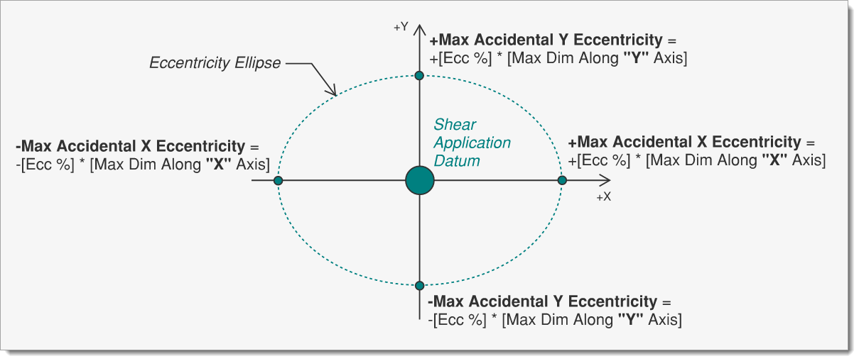
The X- and Y-direction accidental eccentricities from the Accidental Torsion section define the axes of an ellipse centered at the shear application point. This ellipse represents all possible load locations that account for the full range of accidental eccentricity.
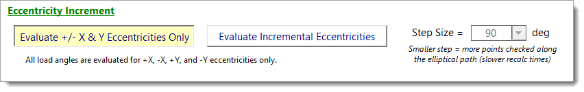
The Eccentricity Increment sets the angular step size (in degrees) used to subdivide the ellipse into discrete load application points. Smaller steps create more load cases and a finer resolution; larger steps reduce the number of cases.
Evaluate +/- X & Y Eccentricities Only
Applies loads at four discrete positions: +Max Accidental X Eccentricity, -Max Accidental X Eccentricity, +Max Accidental Y Eccentricity, and -Max Accidental Y Eccentricity (i.e., the poles of the eccentricity ellipse).
This matches a traditional code-based approach of checking maximum offsets in each principal direction.
Example:
Location of Shear Application: X = 50 ft, Y = 25 ft
Max Accidental X Eccentricity = 5 ft, Max Accidental Y Eccentricity = 2.5 ft
This gives the following load application points:
+Max Accidental X Eccentricity: eacc,x = 5.00, eacc,y = 0.00, x = 55.00, y = 25.00
+Max Accidental Y Eccentricity: eacc,x = 0.00, eacc,y = 2.50, x = 50.00, y = 27.50
-Max Accidental X Eccentricity: eacc,x = -5.00, eacc,y = 0.00, x = 45.00, y = 25.00
-Max Accidental Y Eccentricity: eacc,x = 0.00, eacc,y = -2.50, x = 50.00, y = 22.50
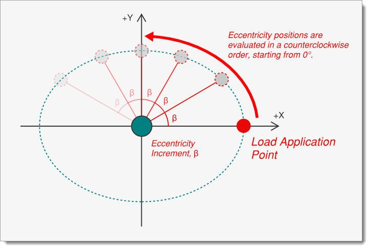
Evaluate Incremental Eccentricities
Applies loads at multiple points along the eccentricity ellipse, using the specified angular increment. This method evaluates a continuous range of eccentricity positions for a more detailed torsional assessment.
The accidental eccentricity and point of load application used for each step at angle θ can be generically described as:
Example:
Location of Shear Application: X = 50 ft, Y = 25 ft
Max Accidental X Eccentricity = 5 ft, Max Accidental Y Eccentricity = 2.5 ft
Eccentricity Increment: 45 degrees
This produces the following load application points:
Eccentricity Increment Step = 0°: eacc,x = 5.00, eacc,y = 0.00, x = 55.00, y = 25.00
Eccentricity Increment Step = 45°: eacc,x = 3.54, eacc,y = 1.77, x = 53.54, y = 26.77
Eccentricity Increment Step = 90°: eacc,x = 0.00, eacc,y = 2.50, x = 50.00, y = 27.50
Eccentricity Increment Step = 135°: eacc,x = -3.54, eacc,y = 1.77, x = 46.46, y = 26.77
Eccentricity Increment Step = 180°: eacc,x = -5.00, eacc,y = 0.00, x = 45.00, y = 25.00
Eccentricity Increment Step = 225°: eacc,x = -3.54, eacc,y = -1.77, x = 46.46, y = 23.23
Eccentricity Increment Step = 270°: eacc,x = 0.00, eacc,y = -2.50, x = 50.00, y = 22.50
Eccentricity Increment Step = 315°: eacc,x = 3.54, eacc,y = -1.77, x = 53.54, y = 23.23
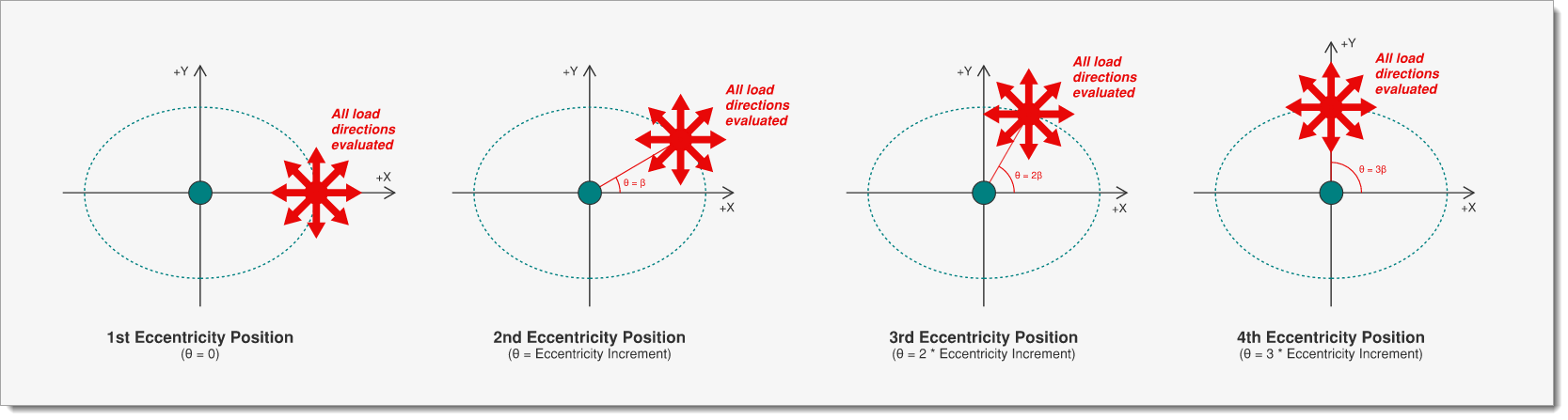
How Load Direction and Eccentricity Increment Work Together
The Load Direction settings controls the direction of the applied lateral force, while the Eccentricity Increment controls the position of that force around the eccentricity ellipse. The module evaluates every combination of these two settings, producing a broad set of load cases from which the maximum forces on each resisting element can be identified.
Example:
If the Load Direction is specified at 30 degree increments and the Eccentricity Increment is 15 degrees, the program evaluates:
•360° / 30° = 12 load directions per eccentricity position
•360° / 15° = 24 eccentricity positions
This results in 12 * 24 = 288 total rigid diaphragm analyses of force distribution to the resisting elements.
Resisting Elements
This tab is used to define the elements that make up the lateral force resisting system. There are three types of resisting elements: Walls, Bending Members, and Generic Resisting Elements. Each type has its own subtab where the specific properties and stiffness parameters are entered.
All subtabs share a common layout consisting of:
Copy, Add, & Delete Buttons
Use these buttons to create new resisting elements, duplicate an existing element, or remove an element from the list.
•Add creates a blank entry for a new element.
•Copy duplicates the currently selected element’s data, which can then be edited.
•Delete removes the selected element from the list.
Element Table
This table lists all resisting elements defined in the current subtab and provides a summary of their input data.
Element Input Data
This area contains the detailed input fields for the selected element, including geometry, material properties, orientation, and end fixity. The specific fields available depend on the element type:
Walls
Use the Walls tab to define a wall as a resisting element. Walls must be rectangular in plan and have a non-zero height.
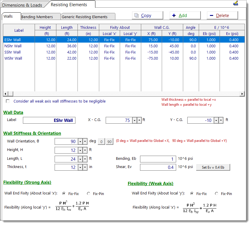
Wall Data
Label: User-defined name for the wall.
X – C.G.: X-coordinate of the wall’s centroid in the global coordinate system (ft).
Y – C.G.: Y-coordinate of the wall’s centroid in the global coordinate system (ft).
Wall Stiffness & Orientation
Wall Orientation, θ: Angle of the wall’s local +y axis (i.e. strong axis) relative to the global +X-axis (0° = wall parallel to global X, 90° = wall parallel to global Y).
NOTE: The wall’s local y axis is parallel to its length dimension; the local x axis is parallel to its thickness dimension.
Height, H: Vertical height of the wall (ft).
Length, L: Horizontal length of the wall in plan (ft), parallel to the wall’s local y axis.
Thickness, t: Thickness of the wall (in), parallel to the wall’s local x axis.
Bending, Eb: Modulus of elasticity for bending stiffness (*106 psi). For example, a value of '1' means Eb = 1,000,000 psi.
Shear, Ev: Modulus of elasticity for shear stiffness (*106 psi). For example, a value of '0.4' means Eb = 400,000 psi.
NOTE: The shear modulus Ev (sometimes also represented as G) of cementitious materials is often estimated as Ev = 0.4 * Eb. This estimate is provided as a convenience in the module but may be overridden with a user-defined value.
For concrete, ACI 318 does not formally define Ev, but it does present this as a reasonable approximation in Commentary R6.6.3.1
For masonry, TMS 402 includes the same approximation in Table 4.2.2.
Flexibility
Wall End Fixity (About local 'x'): End boundary condition for in-plane (strong axis) loading (i.e. loading along local +y / about local +x).
Wall End Fixity (About local 'y'): End boundary condition for out-of-plane (weak axis) loading (i.e. loading along local +x / about local +y).
Fix-Fix: Both ends restrained. The flexibility for a 1-kip unit load is calculated using the following equations:
Fix-Pin: One end fixed, one pinned. The flexibility for a 1-kip unit load is calculated using the following equations:
NOTE: For more information on these flexibility equations, see Torsional Analysis of Rigid Diaphragm Theory - Displacement Behavior of Wall Elements.
Consider all weak axis wall stiffnesses to be negligible: When enabled, the wall is modeled with infinite flexibility in the weak direction (out-of-plane). The flexibility and stiffness will display as “Neglect” on the Resisting Element Data tab.
Bending Members
Use the Bending Members tab to define a bending member (such as a column) as a resisting element. This will be a linear member whose stiffness is specified simply by its X and Y axis moments of inertia.
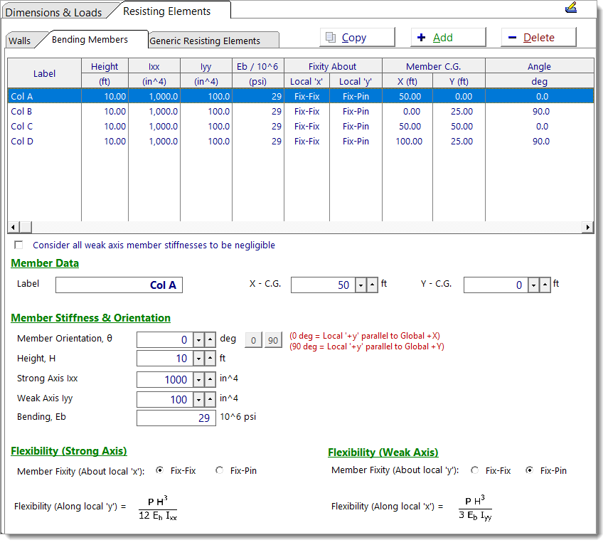
Member Data
Label: User-defined name for the bending member.
X – C.G.: X-coordinate of the bending member’s centroid in the global coordinate system (ft).
Y – C.G.: Y-coordinate of the bending member’s centroid in the global coordinate system (ft).
Member Stiffness & Orientation
Member Orientation, θ: Angle of the member’s local +y axis (i.e. strong axis) relative to the global +X-axis (0° = local +y parallel to global +X, 90° = local +y parallel to global +Y).
Height, H: Vertical height of the member (ft).
Strong Axis Ixx: Moment of inertia about the members local +x axis (in4).
Weal Axis Iyy: Moment of inertia about the members local +y axis (in4).
Bending, Eb: Modulus of elasticity for bending stiffness (*106 psi). For example, a value of '29' means Eb = 29,000,000 psi.
Flexibility
Member Fixity (About local 'x'): End boundary condition for loading in the member's strong direction (i.e. along local +y / about local +x).
Member Fixity (About local 'y'): End boundary condition for loading in the member's weak direction (i.e. along local +x / about local +y).
Fix-Fix: Both ends restrained. The flexibility for a 1-kip unit load is calculated using the following equations:
Fix-Pin: One end fixed, one pinned. The flexibility for a 1-kip unit load is calculated using the following equations:
NOTE: For bending members, flexural deformation dominates the overall behavior and shear deformation is neglected. For more information on these flexibility equations, see Torsional Analysis of Rigid Diaphragm Theory - Displacement Behavior of Wall Elements.
Consider all weak axis member stiffnesses to be negligible: When enabled, the bending member is modeled with infinite flexibility in the weak direction. The flexibility and stiffness will display as “Neglect” on the Resisting Element Data tab.
Generic Resisting Elements
Use the Generic Resisting Elements tab to define a resisting element with user-specified stiffness. This option is intended for complex systems, such as braced or moment frames, where flexibility/stiffness has been determined from another analysis.
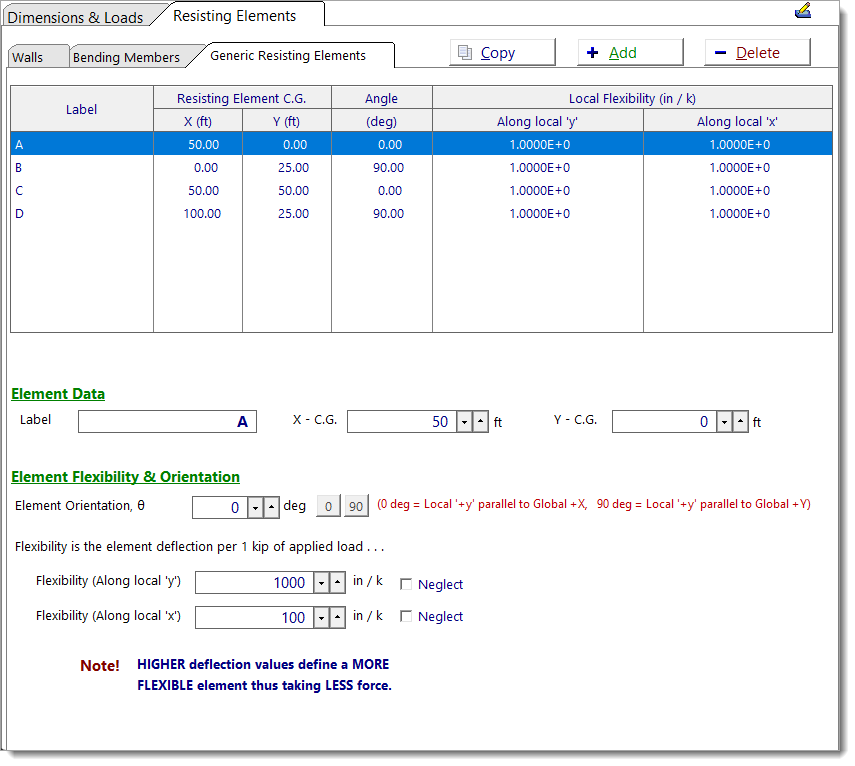
Element Data
Label: User-defined name for the generic resisting element.
X – C.G.: X-coordinate of the element’s centroid in the global coordinate system (ft).
Y – C.G.: Y-coordinate of the element’s centroid in the global coordinate system (ft).
Element Flexibility & Orientation
Element Orientation, θ: Angle of the element’s local +y axis (i.e. strong axis) relative to the global +X-axis (0° = local +y parallel to global +X, 90° = local +y parallel to global +Y).
Flexibility (Along local 'y'): Flexibility of the element along its local +y axis, expressed as the deflection produced by a unit 1-kip load as determined from another analysis.
Flexibility (Along local 'x'): Flexibility of the element along its local +x axis, expressed as the deflection produced by a unit 1-kip load as determined from another analysis.
Neglect: When enabled, the element is modeled with infinite flexibility in the associated direction. The respective flexibility and stiffness will display as “Neglect” on the Resisting Element Data tab.
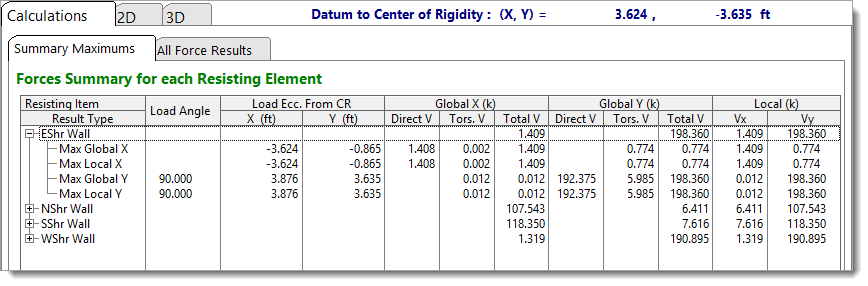
Summary Maximums
The Summary Maximums tab lists the peak global X and Y forces for each resisting element, along with the maximum shear forces in the element’s local major (Vy) and minor (Vx) directions.
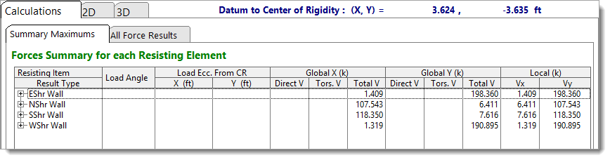
Clicking the [+] icon next to an element name expands the entry to show additional details. Since the maximum global and local forces along each axis may occur under different loading conditions, the expanded view also reports the load direction and eccentricity at which each maximum value occurs.
All Force Results
The All Force Results tab displays the full set of calculated forces for each resisting element. Results are shown in a tree structure, and clicking the [+] icon next to an element name expands its result set.
For example, in the image below, expanding the wall labeled "SShr Wall" reveals multiple lines labeled 0 deg, 15 deg, 30 deg, etc. Each line corresponds to a lateral load applied at a specific load angle as described under Load Direction.
Within each load-angle group, the accidental eccentricity values (Acc X and Acc Y) change to reflect different load application points along the accidental eccentricity ellipse as described under Eccentricity Increment.
A note at the top of the table indicates that the analysis uses 90-degree increments for the Eccentricity Increment, meaning there will be 4 entries for load application point (360 degrees / 90 degrees = 4). Additionally, the load direction varies in 15-degree increments, so scrolling further reveals results for other applied load angles.
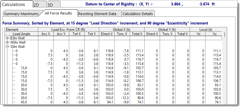
The algebraic signs of the direct and torsional shear components are relative to the global Cartesian coordinate system: Global +X acts to the right on screen, and Global +Y acts upward. These values represent diaphragm forces applied at the top of each resisting element. To determine base reactions, invert the sign of each value.
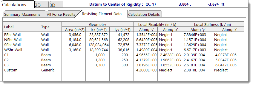
Resisting Element Data
The Resisting Element Data tab consolidates all resisting elements, including Walls, Bending Members, and Generic Resisting Elements, into a single table. It displays the calculated cross-sectional properties (such as area and moments of inertia), along with the corresponding local flexibility and stiffness values in both the X and Y directions. If stiffness along a local axis has been set to be neglected, the word “Neglect” will appear in the relevant flexibility and stiffness columns.
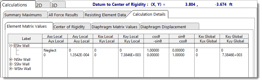
Calculation Details
The Calculation Details tab provides detailed calculations and intermediate results that are used to generate the outputs shown in the All Force Results and Summary Maximums tabs.
Element Matrix Values
The Element Matrix Values tab displays the local 2x2 flexibility and stiffness matrices, the transformation matrices, and the resulting global stiffness matrices for each resisting element.
For additional background on these values, refer to theTorsional Analysis of Rigid Diaphragm Theory documentation, specifically the Resisting Element Local Stiffness and Resisting Element Global Stiffness and Force Transformation topics.
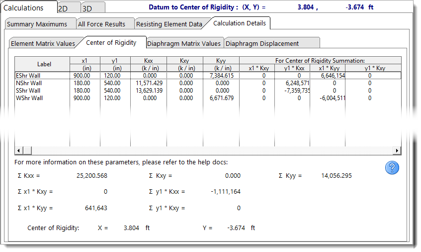
Center of Rigidity
The Center of Rigidity tab displays the individual components and summation terms used to calculate the center of rigidity, including each element’s location and stiffness contributions.
For additional background on these values, refer to theTorsional Analysis of Rigid Diaphragm Theory documentation, specifically the Center of Rigidity and topic.
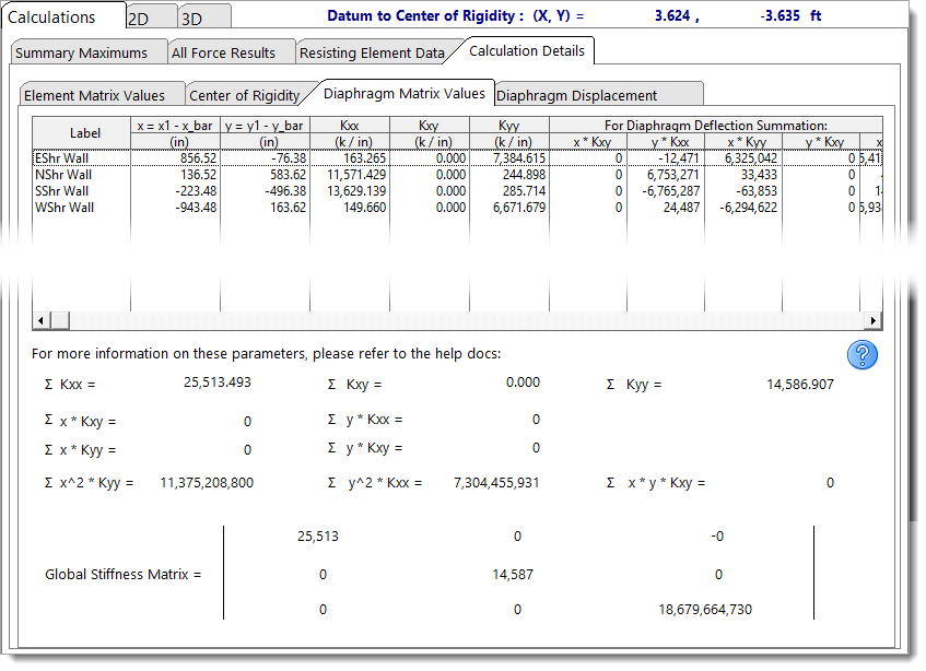
Diaphragm Matrix Values
The Diaphragm Matrix Values tab presents the individual components and summation terms used to calculate the global stiffness matrix for the rigid diaphragm.
For additional background on these values, refer to theTorsional Analysis of Rigid Diaphragm Theory documentation, specifically the Rigid Diaphragm Global Stiffness Matrix and topic.
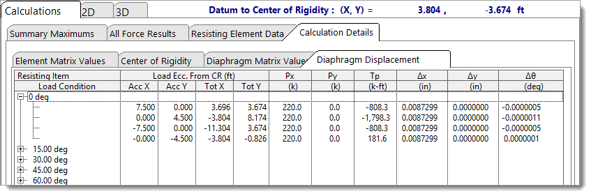
Diaphragm Displacement
The Diaphragm Displacement tab reports the load eccentricities relative to the center of rigidity, the applied lateral forces and torsional moments for each load condition or load angle, and the resulting diaphragm displacements and rotations.
For additional background on these values, refer to theTorsional Analysis of Rigid Diaphragm Theory documentation, specifically the Rigid Diaphragm Global Stiffness Matrix and topic.
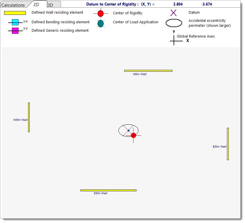
2D Sketch
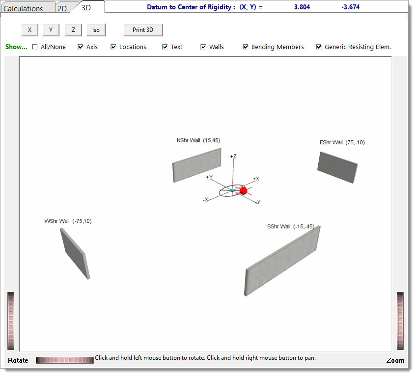
3D Rendering
 <
<