Navigation:  Step-By-Step Examples > Example 1: A Cantilever Beam

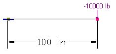
Problem Description

A 100-inch long cantilever beam is subjected to a tip load of -10,000 lbs.

 

Material properties: E = 2.9e7 psi, ν = 0.3

 

Section properties: Ix = 200 in^4, Ay = 8.33333 in^2

 

Analyze the beam for the following two cases:

a). Model the beam with one frame element.  Verify the vertical displacement and rotation at the tip of the beam, with/without the shear deformation considered.  

b). Model the beam with 1,000; 10,000; 20,000; and 50,000 members.  Analyze the each model with the 64-bit and 128-bit floating point solver.  Compare the vertical displacements without shear deformation considered.

 

 

Suggested Modeling Steps

▪Set proper units from Settings and Tools > Units & Precisions.

▪Generate the beam geometry by Create > Templates > Rectangular Frames.  For example, to generate 1,000 members (each with 0.1 inch in length), enter a distance list of “1000@0.1” in the X direction.  Do not enter anything for the Y and Z directions.

▪Select all members, define and assign the material properties by Modify > Member Properties > Materials. Make sure “Assign active material to currently selected elements” is checked in the dialog box.

▪Select all members, define and assign the section properties by Modify > Member Properties > Sections.  Make sure “Assign active section to currently selected members” is checked in the dialog box.

▪Press ESC key to unselect all nodes and elements.  Select the first node by Create > Select > Select Nodes, and assign it a fixed support by Create > Boundary Conditions > Support.

▪Select the last node by Create > Select > Select Nodes, and assign it a nodal load of -10,000 lb in the global Y direction.  The load is assigned to the built-in load case called “Default”.  ENERCALC 3D also provides a load combination called “Default” which is 1.0 * “Default” load case by default.

▪Set the analysis options by Analysis > Analysis Options.  Choose the model type “2D Frame”. Check or uncheck “Consider shear deformation on members”.  Select the 64-bit or 128-bit floating point skyline solver.

 

Results

The displacement at the tip of the beam may be calculated by hand as follows:

psi

in (shear deformation ignored)

in (shear deformation considered)

radian

 

The following table shows the tip displacement and rotation of the beam modeled with one element.  The comparison between the program and theoretical results is excellent.

 

 

The following table shows the tip displacements of the beam modeled with 1000; 10,000; 20,000; and 50,000 elements.  Shear deformations are ignored.  The four models are solved with the 64-bit (skyline) floating point and the 128-bit floating point solvers of the program.

 

 

Comments

This is probably the simplest structural model that can be solved by either hand or an analysis program.  However, it could be turned into a very challenging numerical problem as shown in the example.  The standard 64-bit floating point (double precision) solver, which is the predominant and only solver in almost all other analysis programs, tends to deteriorate in solution accuracy as the number of elements increases.  In the example, the 64-bit floating point becomes unstable after 10,000 elements.  For the model with 50,000 elements, some diagonal terms in the global stiffness matrix even become negative during factorization process. The solver has to terminate and the solution is not obtainable anymore. Getting no results is better than getting incorrect results.  Try this model on your familiar structural analysis software!

 

ENERCALC 3D implements a unique 128-bit floating point (quad precision) solver that is extremely accurate and stable in solution.  Its superiority is demonstrated in that it gives consistent and correct results up to 50,000 elements. You are encouraged to try even more elements to solve this problem.  Just make sure you have enough computer memory to handle large models.  If you generate a large model by splitting existing members, make sure you renumber the nodes after splitting to minimize the bandwidth in the model.