Fluid Loads (on Shells) |
  
|
Fluid Loads (on Shells) |
|
The Fluid Loads command provides a convenient way to apply a linear varying surface load on a selected mesh of shells. The load will be applied in the local z direction of all selected shells, that is, perpendicular to the shell and in the positive or negative local z direction based on the algebraic sign of the load value.
Note that although the load can vary in intensity, it will be discretized such that the load will be uniform on each individual shell.
Graphical Method
The command is accessed by clicking Create > Generate Loads > Fluid Loads, which opens the Fluid Load dialog.
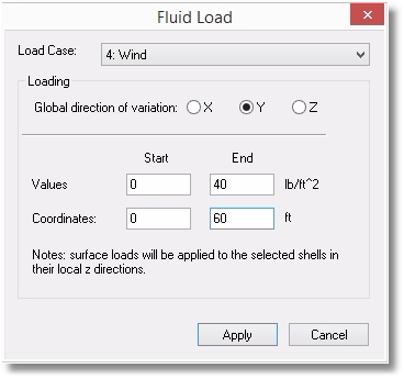
Select the load case with which the Fluid Load is to be associated.
The actual loading is specified as three components: a global direction of variation, a starting coordinate with load intensity and an ending coordinate with load intensity.
Tabular Method
The tables are useful for reviewing and editing the loads produced by the Fluid Loads command, because they get generated as surface loads on shells. But the tables don't have the power to generate Fluid Loads of varying magnitudes on multiple shells.
Clicking Tables > Surface Loads opens the Surface Loads table.
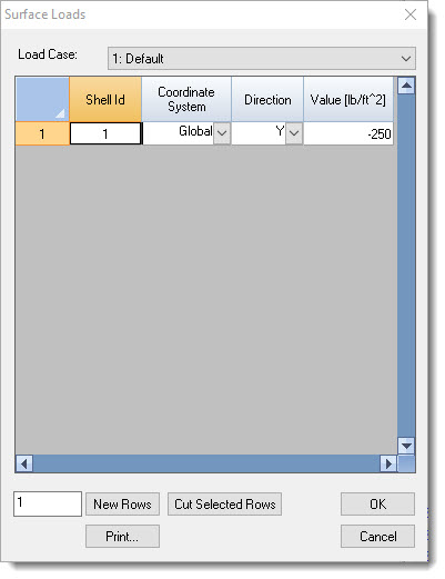
This table displays all loads applied to shells, including those generated by the Fluid Loads command. Any of the data can be edited in this table, and new data can be created by manually inserting new rows. But remember that the real utility of the Fluid Loads command is its ability to create varying loads on many shells automatically.
